Locating and Filling Missing Words in Sentences
Sat 05 Mar 2016 by Tianlong Song Tags Natural Language ProcessingThere has been many occasions that we have incomplete sentences that are needed to completed. One example is that in speech recognition noisy environment can lead to unrecognizable words, but we still hope to recover and understand the complete sentence (e.g., by inference); another example is sentence completion questions that appear in language tests (e.g., SAT, GRE, etc.).
What are Exactly the Problem?
Generally, the problem we are aiming to solve is locating and filling any missing words in incomplete sentences. However, this problem seems too ambitious so far, and we direct ourselves to a simplified version of this problem. To simplify the problem, we assume that there is only one missing word in a sentence, and the missing word is neither the first word nor the last word of the sentence. This problem originally comes from here.
Locating the Missing Word
Two approaches are presented here so as to locate the missing word.
N-gram Model
For a given training data set, define \(C(w_1,w_2)\) as the number of occurrences of the bigram pattern \((w_1,w_2)\), and \(C(w_1,w,w_2)\) the number of occurrences of the trigram pattern \((w_1,w,w_2)\). Then, the number of occurrences of the pattern, where there is one and only one word between \(w_1\) and \(w_2\), can be calculated by
where \(V\) is the vocabulary.
Consider a particular location, \(l\), of an incomplete sentence of length \(L\), and let \(w_l\) be the \(l\)th word in the sentence. \(D(w_{l-1},w_{l})\) would be the number of positive votes from the training data set for missing word at this location, while \(C(w_{l-1},w_{l})\) would be correspondingly the number of negative votes. We define the score indicating there is a missing word at location \(l\) as
where \(\gamma\) is a small positive constant. Hence, the missing word location can be identified by
Note that in (\ref{Eqn:Score}), if we set \(\gamma=0\), the left part would be exactly the percentage of positive votes for missing word at that location, and the right part is the percentage of negative votes. It seems a fairly reasonable score, then why do we still need a positive \(\gamma\)? The underlying reason is that intuitively the more number of votes for a particular decision, the more confident we are on that decision. This trend is reflected in a positive \(\gamma\), which can be viewed as sparse vote penalty and is useful in breaking ties in the missing word location voting. That is, if we have exactly the same ratio of positive votes relative to negative votes for two candidate locations, e.g., 80 positive votes v.s. 20 negative votes for location A, and 8 positive votes v.s. 2 negative votes for location B, we would believe that location A is more likely to be the missing word location compared with location B.
Word Distance Statistics (WDS)
In view of the fact that the statistics of the two words immediately adjacent to a given location contribute a lot in deciding whether the location has a word missing, we tentatively guess that all the words within a window centered at that location would more or less contribute some information as well. As a result, we introduce the concept of word distance statistics (WDS).
More specifically, we use \(\widetilde{C}(w_1,w_2,m)\) to denote the number of occurrences of the pattern, where there is exactly \(m\) words between \(w_1\) and \(w_2\), i.e., the word distance of \(w_1\) and \(w_2\) is \(m\). For a given location \(l\) in an incomplete sentence and a word window size \(W\), we are interested in the word distance statistics of each word pair, in which one word \(w_i\) is on the left of the location \(l\), and the other word \(w_j\) is on the right, as illustrated in Fig. 1.
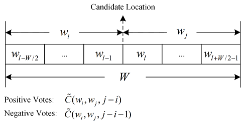
Formally, for any \(l-W/2 \leq i \leq l-1\) and \(l \leq j \leq l+W/2-1\), \(\widetilde{C}(w_i,w_j,j-i)\) would be the number of positive votes for missing word at this location, while \(\widetilde{C}(w_i,w_j,j-i-1)\) is the number of negative votes. Applying the idea in (\ref{Eqn:Score}), for each word pair \((w_i,w_j)\), we extract its feature as the score indicating there is a missing word at location \(l\), i.e.,
As a special example, let \(i=l-1\) and \(j=l\), (\ref{Eqn:ScoreGeneralized}) would be reduced to (\ref{Eqn:Score}).
To find the missing word location, we need to assign different weights to the extracted features, \(S_l(i,j)\). Then, the missing word location can be determined by
where the weight, \(v(i,j)\), should be monotonically decreasing with respect to \(|j-i|\).
Filling the Missing Word
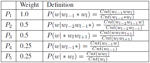
To find the most probable word in the given missing word location, we take into account five conditional probabilities, as shown in Table 1, to explore the statistical connection between the candidate words and the surrounding words at the missing word location. Ultimately, the most probable missing word can be determined by
where \(B\) is the candidate word space (detailed here), and the weight \(v_i\) is used to reflect the importance of each conditional probability in contributing to the final score.
Experimental Results
The training data contains \(30,301,028\) complete sentences, of which the average sentence length is approximately \(25\). In the vocabulary with a size of \(2,425,337\), \(14,216\) words that have occurred in at least \(0.1\%\) of total sentences are labeled as high-frequency words, and the remaining \(58,417,315\) words are labeled as 'UNKA'. To perform the cross validation, in our experiments, the training data is splitted into two part, TRAIN and DEV. The TRAIN set is used to train our models, and the DEV set is applied to test our models.
Missing Word Location
Table 2 shows the estimation accuracy of the missing word locations for the two proposed approaches, N-gram and WDS. For comparison, we list the corresponding probabilities by chance as well. Each entry shows the probabilities that the correct location is included in the ranked candidate location list returned by each approach, where the list size varies from \(1\) to \(10\). The sparse vote penalty coefficient, \(\gamma\), is set to 0.01. In the WDS approach, we consider a word window size \(W=4\), i.e., four pairs of words are taken into account.
| Top 1 | Top 2 | Top 3 | Top 5 | Top 10 | |
|---|---|---|---|---|---|
| Chance | 4% | 8% | 12% | 20% | 40% |
| N-gram | 51.47% | 63.70% | 71.00% | 80.26% | 91.54% |
| WDS | 52.06% | 64.50% | 71.76% | 80.91% | 91.93% |
Missing Word Filling
Table 3 shows the accuracies of filling the missing word given the location. Each row of the second column shows the probability that the correct word is included in the ranked candidate words list returned by the proposed approach.
| Top 1 | Top 2 | Top 3 | Top 5 | Top 10 | |
|---|---|---|---|---|---|
| Accuracy | 32.15% | 41.49% | 46.23% | 52.02% | 59.15% |
Acknowledgement
I did this project with my partner, Zhe Wang. To see the codes and/or report, click here for more information.