Neural Networks and Deep Learning
Sun 03 Apr 2016 by Tianlong Song Tags Machine Learning Data MiningIt has been a long time since the idea of neural networks was proposed, but it is really during the last few years that neural networks have become widely used. One of the major enablers is the infrastructure with high computational capability (e.g., cloud computing), which makes the training of large and deep (multilayer) neural networks possible. This post is in no way an exhaustive review of neural networks or deep learning, but rather an entry-level introduction excerpted from a very popular book1.
Neural Network (NN) Basics
Let us start with sigmoid neurons, and then find out how they are used in NNs.
Sigmoid Neurons
As the smallest unit in NNs, a sigmoid neuron mimics the behaviour of a real neuron in human neural systems. It takes multiple inputs and generates one single output, as in a process of local or partial decision making. More specifically, given a series of inputs \([x_1,x_2,...]\), a neuron applies the sigmoid function to the weighted sum of the inputs plus a bias, i.e., the output of the neuron is computed as
where \(z=\sum_j{w_jx_j}+b\) is the weighted input to the neuron, and the sigmoid function, \(\sigma(z)=\frac{1}{1+\exp(-z)}\), is to approximate the step function as usually used in binary decision making. A natural question is: why do not we just use the step function? The answer is that the step function is not smooth (not differentiable at origin), which disables the gradient method in model learning. With the smoothed version of the step function, we are safe to relate the change at the output to the weight/bias changes by
The Architecture of NNs
The architecture of a typical NN is depicted in Fig. 1. As shown, the leftmost layer in this network is called the input layer, and the neurons within this layer are called input neurons. The rightmost or output layer contains the output neuron(s). The middle layer is called a hidden layer, since the neurons in this layer are neither inputs nor outputs.
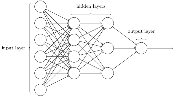
It was proved that NNs with a single hidden layer can be used to approximate any continuous function to any desired precision. Click here to see how. It can be expected that a NN with more neurons/layers could be more accurate in the approximation.
Learning with Gradient Descent
Before training a model, we first need to find a way to quantify how well we are achieving. That is, we need to introduce a cost function. Although there are many cost functions available, we will start with the quadratic cost function, which is defined as
where \(w\) denotes the collection of all weights in the network, \(b\) all the biases, \(n\) is the total number of training inputs, \(a\) is the vector of outputs from the network when \(x\) is input, and the sum is over all training inputs, \(x\).
Applying the gradient descent method, we can learn the weights and biases by
To compute each gradient, we need to take into account all the training input \(x\) in each iteration. However, this slows the learning down if the training data size is large. An idea called stochastic gradient descent (a.k.a., mini-batch learning) can be used to speed up learning. The idea is to estimate the gradient by computing it for a small sample of randomly chosen training inputs.
The Backpropagation Algorithm: How to Compute Gradients of the Cost Function?
So far we have known that the model parameters can be learned by the gradient descent method, but the computation of the gradients can be challenging by itself. Note that the network size and the data size can both be very large. In this section, we will see how the backpropagation algorithm helps compute the gradients efficiently.
Matrix Notation for NNs
For ease of presentation, let us define some notations first.
\(w_{jk}^l\): weight from the \(k\)th neuron in layer \(l-1\) to the \(j\)th neuron in layer \(l\);
\(w^l=\{w_{jk}^l\}\): matrix including all weights from each neuron in layer \(l-1\) to each neuron in layer \(l\);
\(b_j^l\): bias for the \(j\)th neuron in layer \(l\);
\(b^l=\{b_j^l\}\): column vector including all biases for each neuron in layer \(l\);
\(a_j^l=\sigma(\sum_k{w_{jk}^la_k^{l-1}+b_j^l})\): activation of the \(j\)th neuron in layer \(l\);
\(a^l=\{a_j^l\}=\sigma(w^la^{l-1}+b^l)\): column vector including all activations of each neuron in layer \(l\);
\(z_j^l=\sum_k{w_{jk}^la_k^{l-1}+b_j^l}\): weighted input to the \(j\)th neuron in layer \(l\);
\(z^l=\{z_j^l\}=w^la^{l-1}+b^l\): column vector including all weighted inputs to each neuron in layer \(l\);
\(\delta_j^l=\frac{\partial{C}}{\partial{z_j^l}}\): gradient of the cost function w.r.t. the weighted input to the \(j\)th neuron in layer \(l\), \(z_j^l\);
\(\delta^l=\{\delta_j^l\}\): column vector including all gradients of the cost function w.r.t. the weighted input to each neuron in layer \(l\).
Four Fundamental Equations behind Backpropagation
There are four fundamental equations behind backpropagation, which will be explained one by one as below.
First, the gradient of the cost function w.r.t. the weighted input to each neuron in output layer \(L\) can be computed as
where \(\nabla_{a^L}C=\{\frac{\partial{C}}{\partial{a_j^L}}\}\) is defined to be a column vector whose components are the partial derivatives \(\frac{\partial{C}}{\partial{a_j^L}}\), \(\sigma'(z)\) is the first-order derivative of the sigmoid function \(\sigma(z)\), and \(\odot\) represents an element-wise product.
Second, the gradient of the cost function w.r.t. the weighted input to each neuron in layer \(l(l<L)\) can be computed from the results of layer \(l+1\) (backpropagation), i.e.,
Third, the gradient of the cost function w.r.t. each bias can be computed as
Fourth, the gradient of the cost function w.r.t. each weight can be computed as
The four equations above are not straightforward at first sight, but they are all consequences of the chain rule from multivariable calculus. The proof can be found here.
The Backpropagation Algorithm
The backpropagation algorithm essentially includes a feedforward process and a backpropagation process. More specifically, in each iteration:
- Input a mini-batch of \(m\) training examples;
- For each training example \(x\):
- Initialization: set the activations of the input layer by \(a^{x,1}=x\);
- Feedforward: for each \(l=2,3,...,L\), compute \(z^{x,l}=w^la^{x,l-1}+b^l\) and \(a^{x,l}=\sigma(z^{x,l})\);
- Output error: compute the error vector \(\delta^{x,L}=\nabla_{a^L}C_x \odot \sigma'(z^{x,L})\);
- Backpropagate the error: for \(l=L-1,L-2,...,2\), compute \(\delta^{x,l}=((w^{l+1})^T\delta^{x,l+1}) \odot \sigma'(z^{x,l})\).
- Compute gradients and apply the gradient descent method by
\begin{equation} \frac{\partial{C_x}}{\partial{w_{jk}^l}}=\delta_j^{x,l}a_k^{x,l-1},~~\frac{\partial{C_x}}{\partial{b_j^l}}=\delta_j^{x,l},~~w^l=w^l-\frac{\eta}{m}\sum_x{\delta^{x,l}(a^{x,l-1})^T},~~b^l=b^l-\frac{\eta}{m}\sum_x{\delta^{x,l}}. \end{equation}
Deep Learning
Everything seems going well so far! What if our NNs are deep, i.e., with a lot of hidden layers? Typically we expect a deep NN could deliver better performance than shallow ones. Unfortunately it was observed that: for deep NNs, the learning speeds of the first few layers of neurons can be much higher/lower than those of the last few layers, in which case the NNs cannot be well trained. Click here to see why. This is known as vanishing/exploding gradient problem. To resolve this problem, it is suggested that we should resort to convolutional networks.
Convolutional Networks
Convolutional neural networks use three basic ideas: local receptive fields, shared weights, and pooling. A typical convolutional network is depicted in Fig. 2, where the network includes one input layer, one convolutional layer, one pooling layer and one output layer (fully connected). We will try to understand the three ideas using this network as an example.
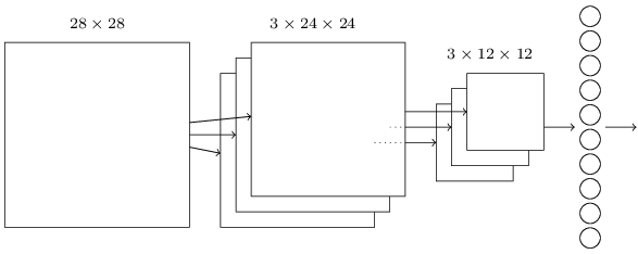
Local receptive fields: Given a 28x28 image as the input layer, instead of directly connecting to all 28x28 pixels, the convolutional layer only connects to small, localized regions (local receptive fields) of the input image in the hope of detecting some localized features. In this example, the small region size is 5x5, so exploring all those regions with a stride length of one results into 24x24 neurons. Here we have three feature maps, so the convolutional layer eventually has 3x24x24 neurons.
Shared weights and biases: We use the same weights and bias for each neuron in a 24x24 feature map. It makes sense to use the same parameters in detecting the same feature but only in different local regions, and it can greatly reduce the number of parameters involved in a convolutional network compared to a fully connected layer.
The pooling layer: A pooling layer is usually used immediately after a convolutional layer. What the pooling layer do is simplify the information in the output from the convolutional layer. In this example, each unit in the pooling layer summarizes a region of 2x2 in the previous convolutional layer, which results into 3x12x12 neurons. The pooling can be a max-pooling (finding the maximum activation of the region to be summarized) or L2 pooling (obtaining the square root of the sum of the squares of the activations in the region to be summarized).
To summarize, a convolutional network tries to detect localized features and at the same time greatly reduces the number of parameters. In principle, we could include any number of convolutional/pooling layers and also fully connected layers in our networks. What is exciting is that the backpropagation algorithm can apply to convolutional networks with only necessary minor modifications.
Does convolutional networks avoid the vanishing/exploding gradient problem? Not really, but it helps us to proceed anyway, e.g., by reducing the number of parameters. The problem can be considerably alleviated by convolutional/pooling layers as well as other techniques, such as powerful regularization, advanced artificial neurons and more training epochs by GPU.
Deep Learning in Practice
It may be not that hard to construct a very basic (deep) NN and achieve a nice performance. However, there are still many techniques that could help to improve the NN's performance. A couple of insightful ideas are listed below, which should be kept in mind if we are working towards a better NN.
- Use more convolutional/pooling layers: reduce the number of parameters and make learning faster;
- Use right cost functions: resolve the problem of learning slow down by the cross-entropy cost function;
- Use regularization: combat overfitting by L2/L1/drop-out regularization;
- Use advanced neurons: for example, tanh neurons and rectified linear units;
- Use good weight initialization: avoid neuron saturation and learn faster;
- Use an expanded training data set: for example, rotate/shift images as new training data in image classification;
- Use an ensemble of NNs: heavy computation, but multiple models beat one;
- Use GPU: gain more training epochs;
Acknowledgement
A large majority of this post comes from Michael Nielsen's book1 entitled "Neural Networks and Deep Learning", which I strongly recommend to anyone interested in discovering how essentially neural networks work.
References
-
M. Nielsen, Neural Networks and Deep Learning, Determination Press, 2015. ↩