Monte Carlo Tree Search and Its Application in AlphaGo

As one of the most important methods in artificial intelligence (AI), especially for playing games, Monte Carlo tree search (MCTS) has received considerable interest due to its spectacular success in the difficult problem of computer Go. In fact, most successful computer Go algorithms are powered by MCTS, including the recent success of Google's AlphaGo¹. This post introduces MCTS and explains how it is used in AlphaGo.

Warm Up: Bandit-Based Methods²

Bandit problems are a well-known class of sequential decision problems, in which one needs to choose among \(K\) actions (e.g. the \(K\) arms of a multi-armed bandit slot machine) in order to maximize the cumulative reward by consistently taking the optimal action. The choice of action is difficult as the underlying reward distributions are unknown, and potential rewards must be estimated based on past observations. This leads to the exploitation-exploration dilemma: one needs to balance the exploitation of the action currently believed to be optimal with the exploration of other actions that currently appear suboptimal but may turn out to be superior in the long run.

The primary goal is to find a policy that can minimize the player's regret after \(n\) plays, which is the difference between: (i) the best possible total reward if the player could at the beginning have the knowledge of the reward distributions that is actually learned afterwards; and (ii) the actual total reward from the \(n\) finished plays. In other words, the regret is the expected loss due to not playing the best bandit. An upper confidence bound (UCB) policy has been proposed, which has an expected logarithmic growth of regret uniformly over the total number of plays \(n\) without any prior knowledge regarding the reward distributions. According to the UCB policy, to minimize his regret, for the current play, the player should choose arm \(j\) that maximizes:

where \(\overline{X}_j\) is the average reward from arm \(j\), \(n_j\) is the number of times arm \(j\) was played and \(n\) is the total number of plays so far. The physical meaning is that: the term \(\overline{X}_j\) encourages the exploitation of higher-rewarded choices, while the term \(\sqrt{\frac{2\ln{n}}{n_j}}\) encourages the exploration of less-visited choices.

Monte Carlo Tree Search (MCTS)²

Let us use the board game as an example. Given a board state, the primary goal would be finding out the best action that should be taken currently, which should naturally be chosen according to some precomputed value of each action. The purpose of MCTS is to approximate the (true) values of actions that may be taken from the current board state. This is achieved by iteratively building a partial search tree.

Four Fundamental Steps in Each Iteration

The basic algorithm involves iteratively building a search tree until some predefined computational budget (e.g., time, memory or iteration constraint) is reached, at which point the search is halted and the best-performing root action returned. Each node in the search tree represents a state, and directed links to child nodes represent actions leading to subsequent states.

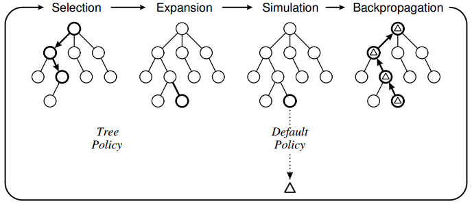
As illustrate in Fig. 1, four steps are applied for each iteration²:

1. Selection: Starting from the root node (i.e., current state), a tree policy for child selection is recursively applied to descend through the tree until an expandable node is reached. A node is expandable if it represents a non-terminal state and has unvisited (i.e., expandable) children.
2. Expansion: For the expandable node we reached in the selection step, one child node is added to expand the tree, according to the available actions.
3. Simulation: A simulation is run from the newly expanded node according to the default policy to produce an outcome (e.g., win or lose when reaching a terminal state).
4. Backpropagation: The simulated result is backpropagated through the selected nodes in the selection step to update their statistics.

There are two essential ideas that should be highlighted here:

• The tree policy for child selection should be able to give the high-value nodes priorities in value approximation, and meanwhile explore the less-visited nodes. This is quite similar to the bandit problem, so we can apply the UCB policy to choose the child node.
• The value of each node is approximated in an incremental way. That is, its initial value is obtained from a random simulation by the default policy (e.g., a win/lose result along a random path), and then refined by the backpropagation steps during the following iterations.

The Full Algorithm Description

Before describing the algorithm, let us define some notations first.

\(s(v)\): the associated state to node \(v\)

\(a(v)\): the incoming action that leads to node \(v\)

\(N(v)\): the visit count of node \(v\)

\(Q(v)\): the vector of total simulation rewards of node \(v\) for all players

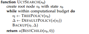
The main procedure of the MCTS algorithm is described below, which essentially executes the four fundamental steps for each iteration until the computational budget is reached. It returns the best action that should be taken for the current state.

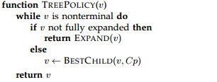
The selection step is described below, which returns the expandable node according to the tree policy.

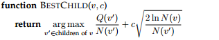
The child selection is described below, which returns the best child of a given node. It essentially applies the UCB method, which uses a constant \(c\) to balance the exploitation with the exploration. It should be noted that there might be multiple players, but the best child is selected as per the interest of the player who is supposed to play in this state.

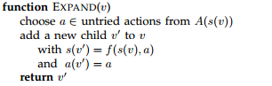
The selected node after the selection step is expanded by choosing one of its unvisited children, and then adding the associated data to the new node. The procedure is described below.

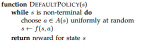
Given the state associating to the newly expanded node, a random simulation is run as indicated below, which finds a random path to a terminal state and returns the simulated reward.

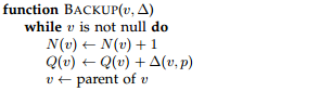
Once the simulated reward of the newly expanded node is obtained, it is backpropagated through the selected nodes in the selection step. The visit counts are updated at the same time.

Recall the board game example, assume that the rewards of winning and losing a game are 1 and 0, respectively. After applying the MCTS algorithm, for each node \(v\) in the tree, \(Q(v)\) would be the number of wins that is accumulated from \(N(v)\) visits of this node, and thus \(\frac{Q(v)}{N(v)}\) would be the winning rate. This is exactly the information we could rely on to choose the best action to take in the current state.

How is MCTS used by Google's AlphaGo?¹

We now understand how MCTS works. Can MCTS be directly applied to computer Go? Yes, but there could be a better way to do that. The reason is that Go is a very high-branching game. Consider the number of all possible sequences of moves, \(b^d\), where \(b\) is the game's breadth (number of legal moves per state, \(b \approx 250\) for Go), and \(d\) is game's depth (game length, \(d \approx 150\) for Go). As a result, exhaustive search is computationally impossible. Applying MCTS to Go in a straightforward way helps, but the benefits of MCTS are not really fully exploited, since the limited number of simulations could only scratch the surface of the giant search space.

Aided by the useful information learned by two deep convolutional neural networks (a.k.a., deep learning), policy network and value network, Google's AlphaGo applies MCTS in an innovative way.

• First, for the tree policy to select child, instead of using the UCB method, AlphaGo takes into account the prior probability of actions learned by the policy network. More specifically, for node \(v_0\), the child \(v\) is selected by maximizing
  \begin{equation} \frac{Q(v)}{N(v)}+\frac{P(v|v_0)}{1+N(v)}, \end{equation}
  where \(P(v|v_0)\) is the prior probability that is provided by the policy network. This greatly improves the child selection policy, and thus grants more professional moves (e.g., by human experts) priorities in MCTS simulation.
• Second, for the default policy to evaluate expanded nodes, AlphaGo combines the outcomes from simulation steps and node values learned by the value network, and their weights are balanced by a constant \(\lambda\).

Note that both the policy network and value network are trained offline, which greatly reduces the time cost in a real-time contest.

Acknowledgement

A large majority of this post, including Fig. 1 and the pseudo codes, comes from the survey paper². More details about MCTS and its variants can be found there.

References